Box-Counting dimension of point datasets

Pramit Ghosh

2024-07-26

Overview

This vignette illustrates the use of this package for calculating the Box-Counting Dimension of point features such as those sf objects with geometry type MULTIPOINT.

For sf objects with geometry type POINT, a Box-Counting dimension cannot be calculated and is (trivially) equal to 0.

Examples

In the following examples, the Box-Counting Dimension will be calculated for both arbitrary MULTIPOINT features with theoretically known fractal dimensions as well as for real-world datasets.

# Loading pre-requisite packages
library(sf)
#> Linking to GEOS 3.10.2, GDAL 3.4.1, PROJ 8.2.1; sf_use_s2() is TRUE
library(sameSVD)

Features with known Box-Counting dimensions

MULTIPOINT feature with 2 points

two_points = st_sf(st_sfc(c(st_point(c(1, 2)), st_point(c(3, 4))), crs = 3857))
two_points
#> Simple feature collection with 1 feature and 0 fields
#> Geometry type: MULTIPOINT
#> Dimension:     XY
#> Bounding box:  xmin: 1 ymin: 2 xmax: 3 ymax: 4
#> Projected CRS: WGS 84 / Pseudo-Mercator
#>   st_sfc.c.st_point.c.1..2....st_point.c.3..4.....crs...3857.
#> 1                                   MULTIPOINT ((1 2), (3 4))

two_points has the following class memberships

class(two_points)
#> [1] "sf"         "data.frame"

plot(st_geometry(two_points), axes = TRUE)

The Box-Counting dimension of this simple feature can be calculated as follows

bcd(two_points, type = "s", l = seq(0.1, 1, 0.1), plot = TRUE)
#> Generating grids...
#> Counting intersecting cells...
#> Performing simple linear regression to determine Box-Counting dimension...
#> Plotting requested...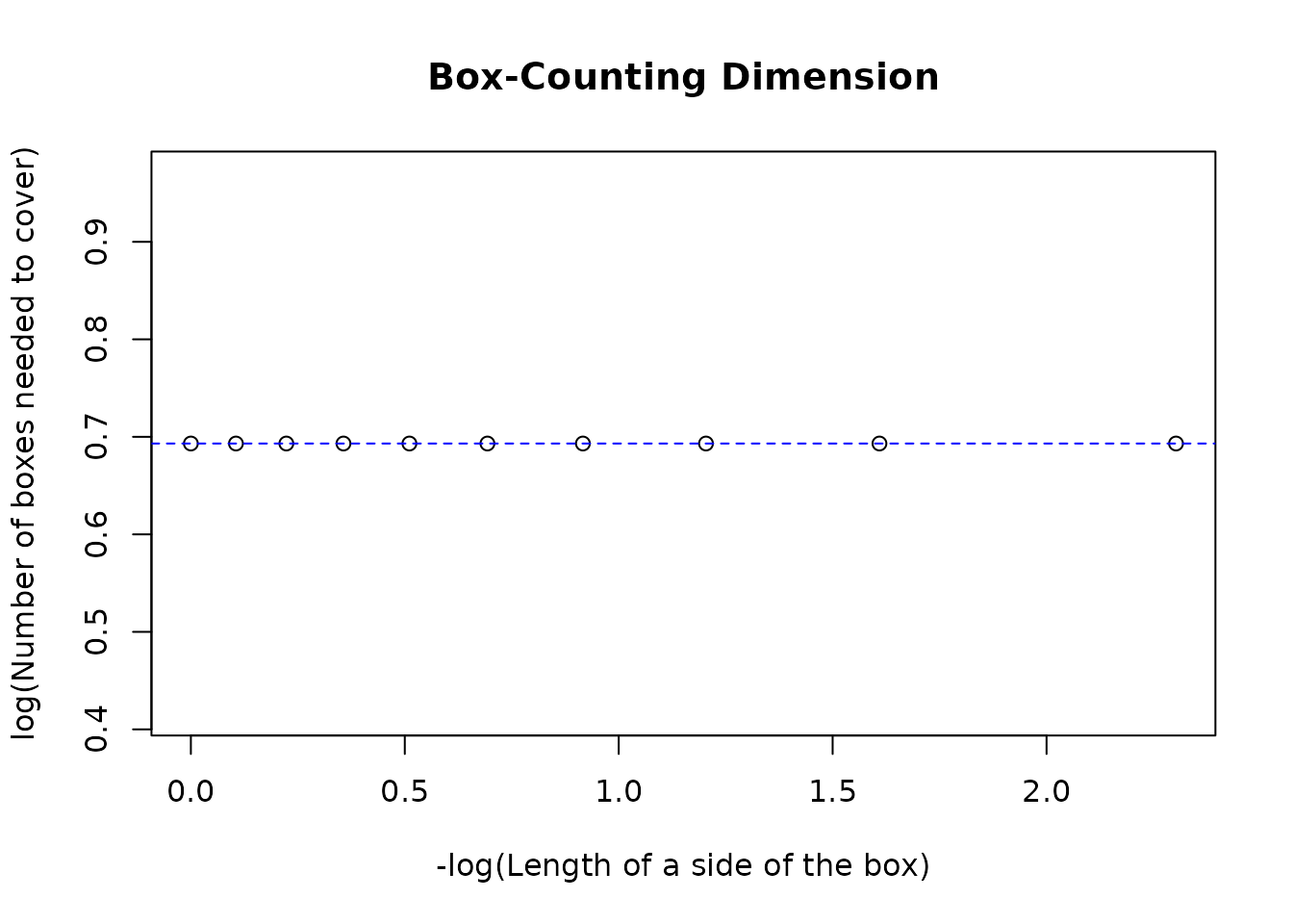

#> Plotting least-squares regression line...
#> [1] 0

The linear regression gives a perfectly horizontal best-fit line indicating a Box-Counting dimension of 0, as expected.

Sierpiński triangle

The Sierpiński triangle is an extensively studied fractal with a theoretically known fractal (Hausdorff) dimension of $log_2(3) = 1.5850$. In this example, a Sierpiński triangle will be generated using a randomized algorithm and its Box-Counting Dimension will be calculated. The following figure shows how the randomized algorithm works and creates the said fractal using discrete points.

By Ederporto - Own work, CC BY-SA 4.0, Link

# Methods to generate a Sierpiński triange
new_points = function(points, last_point, last_vertex = NA)
{
  pt_row = sample(1:dim(points)[1], 1)
  if(!is.na(last_vertex))
  {
    while(pt_row == last_vertex)
      pt_row = sample(1:dim(points)[1], 1)
  }
  mid_pt = c((last_point[1] + points[pt_row, 1])/2, (last_point[2] + points[pt_row, 2])/2)
  list(matrix(mid_pt, nrow = 1), pt_row)
}

The Sierpiński triangle is generated as follows.

# Define initial variables
n = 3 #Create a 3-sided polygon (triangle)
points = matrix(data = c(c(0,0), c(1,0), c(cos(pi/3), sin(pi/3))), ncol = 2, byrow = TRUE, dimnames = list(LETTERS[1:n], c("x", "y"))) #Define vertices of triangle
last_pt = matrix(data = c(0,0), nrow = 1) #Choose a random starting point
max_pts = 20000

# Generate coordinates
sierpinski = list()
length(sierpinski) = max_pts
for(i in 1:max_pts){
  last_pt = new_points(points, last_pt)[[1]]
  sierpinski[[i]] = last_pt
}
sierpinski_pts = matrix(unlist(sierpinski), ncol = 2, byrow = TRUE)

The generated Sierpiński triangle is converted to a sf MULTIPOINT object with a CRS EPSG:3857.

(sierpinski_sf = st_sf(st_sfc(st_multipoint(sierpinski_pts), crs = 3857)))
#> Simple feature collection with 1 feature and 0 fields
#> Geometry type: MULTIPOINT
#> Dimension:     XY
#> Bounding box:  xmin: 0 ymin: 0 xmax: 0.9988957 ymax: 0.8647843
#> Projected CRS: WGS 84 / Pseudo-Mercator
#>   st_sfc.st_multipoint.sierpinski_pts...crs...3857.
#> 1                    MULTIPOINT ((0 0), (0.25 0....
plot(sierpinski_sf, pch = '.', axes = TRUE)

The Box-Counting Dimension of this figure is calculated using bcd() as illustrated below.

bcd(sierpinski_sf, type = "s", l = seq(0.01, 0.1, 0.01), plot = TRUE)
#> Generating grids...
#> Counting intersecting cells...
#> Performing simple linear regression to determine Box-Counting dimension...
#> Plotting requested...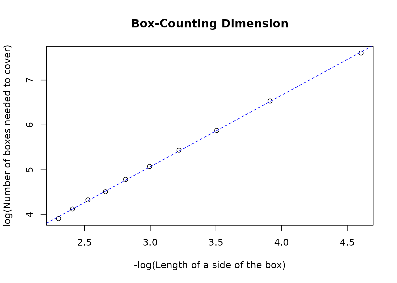

#> Plotting least-squares regression line...
#> [1] 1.593836

The regression gives a Box-Counting dimension of ~1.59 which is very close to the theoretical value.

Other Fractals

Barnsley fern

Barnsley fern is a well-known fractal that was first described by a British mathematician, Michael Barnsley, in 1993. A Barnsley fern is constructed mathematically using a Iterated function system (IFS), a common method to generate fractals.

In an IFS, a fractal is constructed iteratively as the union of several copies of itself. Before performing the union of the set, self-affine transformations are often applied to the component copies by a function system with finite number of contraction mappings. Formally, the IFS is usually expressed using a Hutchinson operator. Let $\{f_i\colon X\to X\mid1\le i\le N\}$ be an IFS - i.e. a set of contractions on set $X$ to itself. Then the operator $H$ is defined over subsets $S\subset X$ as $$H(S)=\bigcup\limits_{i=1}^{N}f_i(S)$$.

Generating the fern programmatically

The finite set of affine transformations are applied stochastically depending on its influence on the generation of the fern.

barnsley_ifs = function(x, y)
{
  xn = 0
  yn = 0
  
  r = runif(1)
  
  if(r < 0.01)
  {
    xn = 0.0
    yn = 0.16 * y
  } else
    if(r < 0.86)
    {
      xn = 0.85 * x + 0.04 * y
      yn = -0.04 * x + 0.85 * y + 1.6
    } else
      if(r < 0.93)
      {
        xn = 0.2 * x - 0.26 * y
        yn = 0.23 * x + 0.22 * y + 1.6
      } else
      {
        xn = -0.15 * x + 0.28 * y
        yn = 0.26 * x + 0.24 * y + 0.44
      }
  
  return(c(xn, yn))
}

max_iterations = 20000
fern = list()
fern[[1]] = c(0, 0)

for(i in 1:max_iterations)
{
  fern[[i+1]] = barnsley_ifs(fern[[i]][1], fern[[i]][2])
}

fern_pts = matrix(unlist(fern), ncol = 2, byrow = TRUE)
(fern_sf = st_sf(st_sfc(st_multipoint(fern_pts), crs = 3857)))
#> Simple feature collection with 1 feature and 0 fields
#> Geometry type: MULTIPOINT
#> Dimension:     XY
#> Bounding box:  xmin: -2.181518 ymin: 0 xmax: 2.652911 ymax: 9.998063
#> Projected CRS: WGS 84 / Pseudo-Mercator
#>   st_sfc.st_multipoint.fern_pts...crs...3857.
#> 1              MULTIPOINT ((0 0), (0 1.6),...
plot(fern_sf, pch = '.', axes = TRUE, col = "forestgreen")

Computing the fractal dimension

The fractal dimension is calculated for the Barnsley fern using bcd().

bcd(fern_sf, type = "s", seq(0.1, 1, 0.1), plot = TRUE)
#> Generating grids...
#> Counting intersecting cells...
#> Performing simple linear regression to determine Box-Counting dimension...
#> Plotting requested...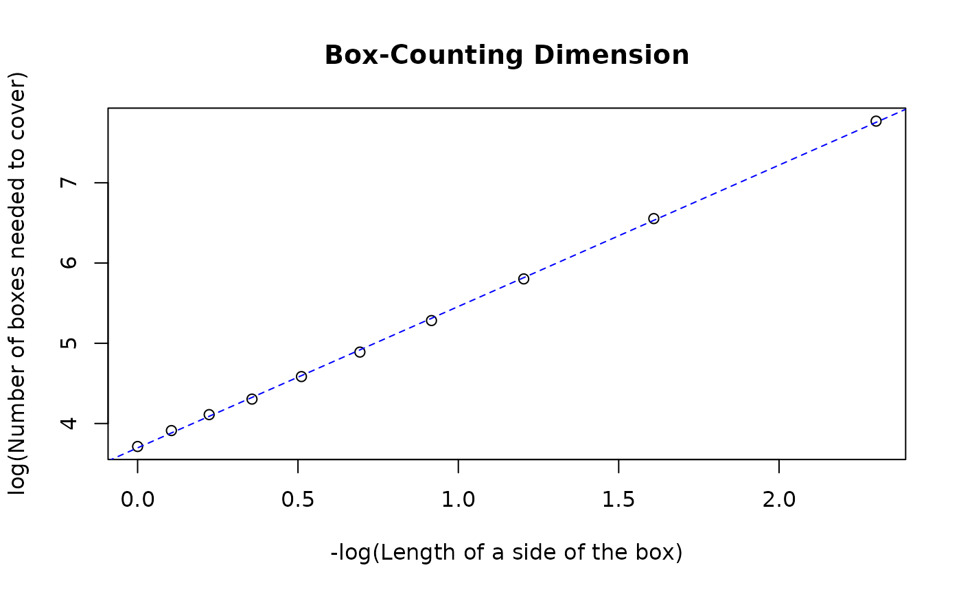

#> Plotting least-squares regression line...
#> [1] 1.761826